SVM

Model: SVM Implementation

Trying out the support vector machine algorithm on the stellar-classification dataset, to successfully predict the target variable.

Preprocess the Data

Code

# import the required libraries
import pandas as pd
import numpy as np
import matplotlib.pyplot as plt
import matplotlib.patches as mpatches

from sklearn.svm import SVC
from sklearn.metrics import accuracy_score
from sklearn.model_selection import train_test_split
from sklearn.preprocessing import StandardScaler
from sklearn.compose import ColumnTransformer
from sklearn.compose import make_column_selector as selector
from sklearn.preprocessing import PowerTransformer
from sklearn.pipeline import Pipeline
from sklearn.preprocessing import OneHotEncoder

import tensorflow as tf

Code

# load in the dataset
# note: uncomment the following lines to download the dataset
# !kaggle datasets download -d fedesoriano/stellar-classification-dataset-sdss17
# !unzip stellar-classification-dataset-sdss17.zip
# !rm stellar-classification-dataset-sdss17.zip
# !echo 'Dataset Downloaded Successfully'

Code

# read in the dataset
stellar = pd.read_csv("star_classification.csv")
stellar.head()

	obj_ID	alpha	delta	u	g	r	i	z	run_ID	rerun_ID	cam_col	field_ID	spec_obj_ID	class	redshift	plate	MJD	fiber_ID
0	1.237661e+18	135.689107	32.494632	23.87882	22.27530	20.39501	19.16573	18.79371	3606	301	2	79	6.543777e+18	GALAXY	0.634794	5812	56354	171
1	1.237665e+18	144.826101	31.274185	24.77759	22.83188	22.58444	21.16812	21.61427	4518	301	5	119	1.176014e+19	GALAXY	0.779136	10445	58158	427
2	1.237661e+18	142.188790	35.582444	25.26307	22.66389	20.60976	19.34857	18.94827	3606	301	2	120	5.152200e+18	GALAXY	0.644195	4576	55592	299
3	1.237663e+18	338.741038	-0.402828	22.13682	23.77656	21.61162	20.50454	19.25010	4192	301	3	214	1.030107e+19	GALAXY	0.932346	9149	58039	775
4	1.237680e+18	345.282593	21.183866	19.43718	17.58028	16.49747	15.97711	15.54461	8102	301	3	137	6.891865e+18	GALAXY	0.116123	6121	56187	842

Code

# statistical overview of the dataset
stellar.info()

<class 'pandas.core.frame.DataFrame'>
RangeIndex: 100000 entries, 0 to 99999
Data columns (total 18 columns):
 #   Column       Non-Null Count   Dtype  
---  ------       --------------   -----  
 0   obj_ID       100000 non-null  float64
 1   alpha        100000 non-null  float64
 2   delta        100000 non-null  float64
 3   u            100000 non-null  float64
 4   g            100000 non-null  float64
 5   r            100000 non-null  float64
 6   i            100000 non-null  float64
 7   z            100000 non-null  float64
 8   run_ID       100000 non-null  int64  
 9   rerun_ID     100000 non-null  int64  
 10  cam_col      100000 non-null  int64  
 11  field_ID     100000 non-null  int64  
 12  spec_obj_ID  100000 non-null  float64
 13  class        100000 non-null  object 
 14  redshift     100000 non-null  float64
 15  plate        100000 non-null  int64  
 16  MJD          100000 non-null  int64  
 17  fiber_ID     100000 non-null  int64  
dtypes: float64(10), int64(7), object(1)
memory usage: 13.7+ MB

Great! Looks like we have no observations with missing values

Code

# closer look at the features

result = {}
features = stellar.columns

for feature in features:
    if stellar[feature].nunique() > 10:
        result[feature] = stellar[feature].nunique()
    else:
        result[feature] = stellar[feature].unique()
result

{'obj_ID': 78053,
 'alpha': 99999,
 'delta': 99999,
 'u': 93748,
 'g': 92651,
 'r': 91901,
 'i': 92019,
 'z': 92007,
 'run_ID': 430,
 'rerun_ID': array([301]),
 'cam_col': array([2, 5, 3, 4, 6, 1]),
 'field_ID': 856,
 'spec_obj_ID': 100000,
 'class': array(['GALAXY', 'QSO', 'STAR'], dtype=object),
 'redshift': 99295,
 'plate': 6284,
 'MJD': 2180,
 'fiber_ID': 1000}

We see that there are 3 values for our traget variable class, namely:

• GALAXY
• QSO
• START

Code

# number of observations
len(stellar)

100000

Code

# reorder the observations based on the class variable
stellar.sort_values('class', axis=0, ascending=True, inplace=True)

Code

# distribution of the classe's observations
# view the layout of the dataset

result = {}
target_labels = stellar['class'].tolist()

for target in target_labels:
    result[target] = -1

for index, obs in enumerate(stellar.values):
    if result[obs[13]] == -1:
        result[obs[13]] = index
result

{'GALAXY': 0, 'QSO': 59445, 'STAR': 78406}

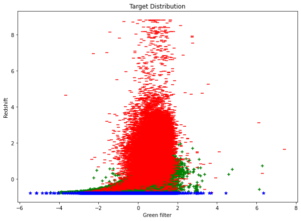
We can now proceed to viewing the distribution of each class in a plot

Code

# visualize using the features: `redshift` and `alpha`
class_labels = stellar['class']
scaled_features = StandardScaler().fit_transform(stellar.drop('class', axis=1))
scaled_stellar = pd.DataFrame(scaled_features, index=stellar.index, columns=(stellar.drop('class', axis=1)).columns)

scaled_stellar['class'] = class_labels
scaled_stellar

	obj_ID	alpha	delta	u	g	r	i	z	run_ID	rerun_ID	cam_col	field_ID	spec_obj_ID	redshift	plate	MJD	fiber_ID	class
0	-0.445634	-0.434604	0.425529	0.059755	0.054926	0.403962	0.046007	0.003937	-0.445535	0.0	-0.952553	-0.718947	0.228609	0.079557	0.228633	0.423203	-1.021342	GALAXY
58230	-1.139298	-0.368710	1.379317	-0.000092	0.031505	0.903290	1.010382	0.053337	-1.139260	0.0	-0.322395	-0.121673	0.731651	0.485616	0.731633	0.802528	0.986019	GALAXY
58228	-1.139298	-0.381213	1.351881	0.045294	0.047447	0.809590	0.974606	0.053707	-1.139260	0.0	-0.322395	-0.161939	0.731256	-0.439343	0.731294	0.805846	-1.516760	GALAXY
58227	-1.070015	0.480361	-1.322346	0.006342	0.031496	0.476575	0.233830	0.007300	-1.070040	0.0	0.307763	-0.584728	-0.378349	-0.092486	-0.378354	-0.141914	0.108945	GALAXY
58226	-1.070015	0.405437	-1.327688	0.112584	0.011681	-0.286498	-0.398618	-0.022590	-1.070040	0.0	0.307763	-0.906853	-1.429054	-0.218501	-1.429064	-1.760957	0.090596	GALAXY
...	...	...	...	...	...	...	...	...	...	...	...	...	...	...	...	...	...	...
46329	-1.092601	0.766323	0.734251	0.045131	0.016127	0.035459	0.100766	0.011344	-1.092435	0.0	-1.582710	-0.953830	1.893737	-0.789715	1.893782	1.470494	-1.509421	STAR
46330	-0.296055	0.617464	0.094237	-0.139661	-0.129397	-2.011636	-1.917283	-0.096359	-0.295898	0.0	-1.582710	3.294198	-0.907107	-0.789845	-0.907096	-0.577640	-0.691063	STAR
46331	-2.124159	-0.701998	-1.226114	0.014384	-0.030837	-0.636966	-0.606623	-0.028993	-2.124116	0.0	-0.322395	-1.088049	0.783445	-0.788944	0.783457	0.626690	-0.335096	STAR
75082	-1.700567	-0.203089	-1.300428	-0.000616	0.010098	0.515621	0.775514	0.049766	-1.700653	0.0	0.937920	-1.020939	-0.457924	-0.787913	-0.457953	-0.174538	1.173177	STAR
68798	1.760822	-1.593640	0.337726	0.050271	0.103026	1.872407	1.077138	0.040500	1.760848	0.0	-0.322395	-0.960541	0.878618	-0.789890	0.878637	1.405246	-0.654366	STAR

100000 rows × 18 columns

Code

x_data = scaled_stellar['i']
y_data = scaled_stellar['redshift']

galaxy_x = x_data[:59445]
galaxy_y = y_data[:59445]

qso_x = x_data[59445:78406]
qso_y = y_data[59445:78406]

star_x = x_data[78406:]
star_y = y_data[78406:]

# create the figure
plt.figure(figsize=(10,7))
plt.scatter(galaxy_x,galaxy_y,marker='+',color='green')
plt.scatter(qso_x,qso_y,marker='_',color='red')
plt.scatter(star_x,star_y,marker='*',color='blue')

plt.title("Target Distribution")
plt.xlabel("Green filter")
plt.ylabel("Redshift")
plt.show()

Feature Engineer Phase

Code

# encode values for class column
stellar.replace({'class': {'GALAXY': 0, 'STAR': 1, 'QSO':2}}, inplace=True)

# remove all columns containing ID at the end
cleaned = stellar.drop(stellar.filter(regex='ID$').columns, axis=1)

# drop the date column
cleaned = stellar.drop('MJD', axis=1)

Code

# make the X and y varialbes (all features)
X_all = cleaned.drop('class', axis=1)
y = cleaned['class']

Code

# keep the 2 features
features = cleaned.columns.tolist()
features.remove('redshift')
features.remove('g')

# make the X and y varialbes
X_specifc = cleaned.drop(features, axis=1)

Code

sc = StandardScaler()
yj = PowerTransformer(method="yeo-johnson")

preprocessor = ColumnTransformer([("norm", yj, selector(dtype_include="number")),
                ("std_encode", sc, selector(dtype_include="number"))
                ])

Build Phase

• Using all features

Code

# initialize an SVC model (all features)
X_train, X_test, y_train, y_test = train_test_split(X_all, y, train_size=0.7, random_state=123)

svc_clf = SVC(kernel='rbf')
svc_model_pipeline = Pipeline(steps=[
  ("preprocessor", preprocessor),
  ("model", svc_clf),
])
# train the model on our dataset
svc_model_pipeline.fit(X_train,y_train)
# store the predictions of the model
y_pred = svc_model_pipeline.predict(X_test)
# evaluate the model on accuracy
print(accuracy_score(y_test,y_pred))

Code

# initialize an SVC model (2 features)
X_train, X_test, y_train, y_test = train_test_split(X_specifc, y, train_size=0.7, random_state=123)

svc_clf = SVC(kernel='rbf')
# train the model on our dataset
svc_model_pipeline = Pipeline(steps=[
  ("preprocessor", preprocessor),
  ("model", svc_clf),
])
svc_model_pipeline.fit(X_train,y_train)
# store the predictions of the model
y_pred = svc_model_pipeline.predict(X_test)
# evaluate the model on accuracy
print(accuracy_score(y_test,y_pred))

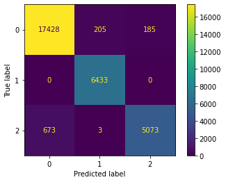
0.9644666666666667

Code

from sklearn.metrics import ConfusionMatrixDisplay
ConfusionMatrixDisplay.from_predictions(y_test, y_pred)

<sklearn.metrics._plot.confusion_matrix.ConfusionMatrixDisplay at 0x14560f730>

Code

# {'class': {'GALAXY': 0, 'STAR': 1, 'QSO':2}}

array([0, 2, 1])

Using Deep Learning

Code

# re-read in the dataset
stellar = pd.read_csv("star_classification.csv")
stellar.head()

	obj_ID	alpha	delta	u	g	r	i	z	run_ID	rerun_ID	cam_col	field_ID	spec_obj_ID	class	redshift	plate	MJD	fiber_ID
0	1.237661e+18	135.689107	32.494632	23.87882	22.27530	20.39501	19.16573	18.79371	3606	301	2	79	6.543777e+18	GALAXY	0.634794	5812	56354	171
1	1.237665e+18	144.826101	31.274185	24.77759	22.83188	22.58444	21.16812	21.61427	4518	301	5	119	1.176014e+19	GALAXY	0.779136	10445	58158	427
2	1.237661e+18	142.188790	35.582444	25.26307	22.66389	20.60976	19.34857	18.94827	3606	301	2	120	5.152200e+18	GALAXY	0.644195	4576	55592	299
3	1.237663e+18	338.741038	-0.402828	22.13682	23.77656	21.61162	20.50454	19.25010	4192	301	3	214	1.030107e+19	GALAXY	0.932346	9149	58039	775
4	1.237680e+18	345.282593	21.183866	19.43718	17.58028	16.49747	15.97711	15.54461	8102	301	3	137	6.891865e+18	GALAXY	0.116123	6121	56187	842

• Feature Engineering

Code

# encode values for class column
stellar.replace({'class': {'GALAXY': 0, 'STAR': 1, 'QSO':2}}, inplace=True)

# remove all columns containing ID at the end
cleaned = stellar.drop(stellar.filter(regex='ID$').columns, axis=1)

# drop the date column
cleaned = cleaned.drop('MJD', axis=1)

# make the X and y varialbes
X = cleaned.drop(['class'], axis=1)
y = cleaned['class']

# split the dataset
X_train, X_test, y_train, y_test = train_test_split(X, y, train_size=0.7, random_state=123)

Code

X_train

	alpha	delta	u	g	r	i	z	cam_col	redshift	plate
52308	48.573323	-0.609684	18.80211	16.75706	15.66640	15.20351	14.80488	2	0.115262	412
27380	260.094957	27.014951	20.26815	18.68293	18.09193	17.86272	17.77524	1	-0.000209	2193
94588	135.477289	37.187920	24.05482	21.67747	20.38921	19.56683	19.27142	2	0.538213	4608
7361	118.180524	9.267706	20.56594	19.53276	19.22361	18.98544	18.89350	4	0.000171	2945
52298	15.024146	4.027261	24.63314	20.48507	18.76055	18.10046	18.07149	1	0.322435	4309
...	...	...	...	...	...	...	...	...	...	...
63206	115.884742	20.139136	18.93230	17.66927	17.21911	16.99153	16.88261	4	0.000022	1263
61404	133.430333	-0.719735	19.83167	19.90659	19.58608	19.57696	19.64975	2	1.309977	12533
17730	255.223294	23.638965	18.99455	18.04598	17.63787	17.44783	17.38555	3	-0.000624	3290
28030	232.458207	36.143802	20.20453	18.46623	17.64739	17.25447	16.98376	3	0.065986	1401
15725	5.646502	3.562572	23.04084	22.26374	22.04945	21.24024	20.42934	6	1.211771	9444

70000 rows × 10 columns

Code

sc = StandardScaler()
yj = PowerTransformer(method="yeo-johnson")

preprocessor = ColumnTransformer([("normalization", yj, selector(dtype_include="number")),
                ("standardization", sc, selector(dtype_include="number")),
                ])

• Building a model

Code

deep_model = tf.keras.Sequential([
    tf.keras.layers.Dense(512, activation='tanh'),
    tf.keras.layers.Dense(64, activation='tanh'),
    tf.keras.layers.Dense(3, activation='softmax')
])

Code

# compile the model
deep_model.compile(
    loss= 'sparse_categorical_crossentropy',
    optimizer= tf.keras.optimizers.SGD(),
    metrics= ['accuracy']
)

Code

# create the pipeline
deep_model_pipeline = Pipeline(steps=[
  ("preprocessor", preprocessor),
  ("model", deep_model),
])

Code

deep_model_pipeline

Pipeline(steps=[('preprocessor',
                 ColumnTransformer(transformers=[('normalization',
                                                  PowerTransformer(),
                                                  <sklearn.compose._column_transformer.make_column_selector object at 0x148b62980>),
                                                 ('standardization',
                                                  StandardScaler(),
                                                  <sklearn.compose._column_transformer.make_column_selector object at 0x148b61b40>)])),
                ('model',
                 <keras.engine.sequential.Sequential object at 0x148b61ab0>)])

In a Jupyter environment, please rerun this cell to show the HTML representation or trust the notebook.
On GitHub, the HTML representation is unable to render, please try loading this page with nbviewer.org.

Code

deep_model.summary()

Model: "sequential_37"
_________________________________________________________________
 Layer (type)                Output Shape              Param #   
=================================================================
 dense_114 (Dense)           (None, 512)               10752     
                                                                 
 dense_115 (Dense)           (None, 64)                32832     
                                                                 
 dense_116 (Dense)           (None, 3)                 195       
                                                                 
=================================================================
Total params: 43,779
Trainable params: 43,779
Non-trainable params: 0
_________________________________________________________________

Code

# fit the model
deep_model_history = deep_model_pipeline.fit(X_train,y_train, model__epochs=10, model__validation_split=0.2)

Epoch 1/10
1750/1750 [==============================] - 13s 7ms/step - loss: 0.2560 - accuracy: 0.9258 - val_loss: 0.1757 - val_accuracy: 0.9546
Epoch 2/10
1750/1750 [==============================] - 15s 9ms/step - loss: 0.1625 - accuracy: 0.9552 - val_loss: 0.1501 - val_accuracy: 0.9616
Epoch 3/10
1750/1750 [==============================] - 15s 8ms/step - loss: 0.1418 - accuracy: 0.9596 - val_loss: 0.1336 - val_accuracy: 0.9631
Epoch 4/10
1750/1750 [==============================] - 16s 9ms/step - loss: 0.1318 - accuracy: 0.9618 - val_loss: 0.1279 - val_accuracy: 0.9635
Epoch 5/10
1750/1750 [==============================] - 20s 11ms/step - loss: 0.1261 - accuracy: 0.9629 - val_loss: 0.1235 - val_accuracy: 0.9656
Epoch 6/10
1750/1750 [==============================] - 21s 12ms/step - loss: 0.1225 - accuracy: 0.9641 - val_loss: 0.1209 - val_accuracy: 0.9651
Epoch 7/10
1750/1750 [==============================] - 21s 12ms/step - loss: 0.1199 - accuracy: 0.9644 - val_loss: 0.1174 - val_accuracy: 0.9665
Epoch 8/10
1750/1750 [==============================] - 23s 13ms/step - loss: 0.1177 - accuracy: 0.9649 - val_loss: 0.1145 - val_accuracy: 0.9672
Epoch 9/10
1750/1750 [==============================] - 25s 14ms/step - loss: 0.1161 - accuracy: 0.9654 - val_loss: 0.1140 - val_accuracy: 0.9674
Epoch 10/10
1750/1750 [==============================] - 26s 15ms/step - loss: 0.1142 - accuracy: 0.9662 - val_loss: 0.1124 - val_accuracy: 0.9677

Code

y_pred = deep_model_pipeline.predict(X_test)
accuracy_score(y_test, y_pred.argmax(axis=-1))

0.9713333333333334